Photogrammetry is the technique which enables the reconstruction and measurement of a scene by means of photographs taken from different positions. First used in 1849 by the Frenchman Aimé Laussedat on the façade of Les Invalides in Paris, the technique has been revolutionised by recent progress in information technology.
The products which can now be generated by photogrammetry include orthophotos, 3D textured models and point clouds. Photogrammetry has numerous advantages, notably including rapid data capture using relatively lightweight equipment, which thus enables surveys of sites which can sometimes be difficult of access.
The technique also has disadvantages, including somewhat variable final accuracy, depending on the quality of the photographs themselves. Moreover, photogrammetry does not work well on textureless surfaces such as glass or polished metal. This difficulty can be overcome by projection of structured light onto the surface.
A camera should not be chosen lightly ! Several specific dimensions should be considered before setting out to take measurements on site.
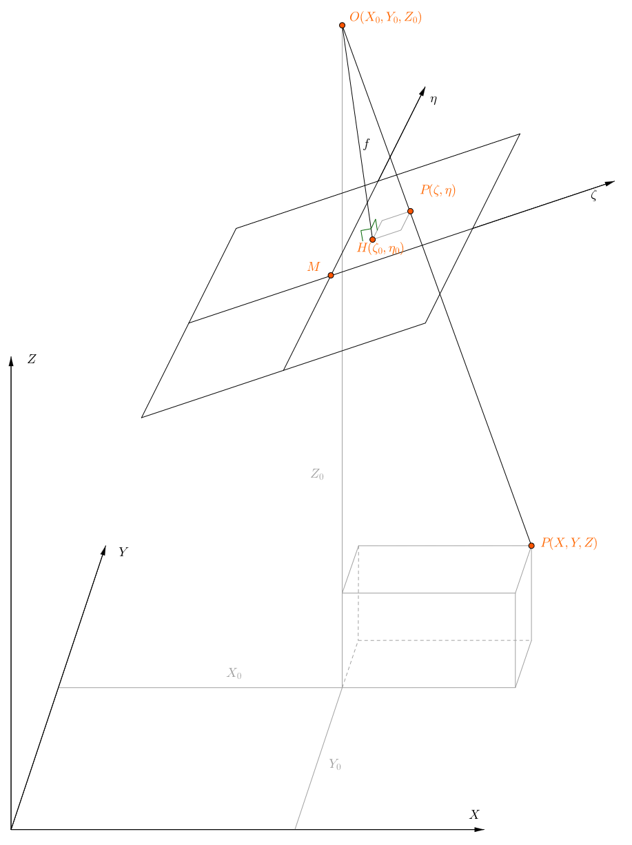
Figure : Basic principle of photogrammetry (Source : Karl Kraus ) :
Here O is the perspective centre of the camera and the focal length is given as f.
Object coordinates are (X, Y, Z), camera coordinates are (ζ, η).
In optics, the focal length or principal distance of a lens is the distance between one of the principal planes within the lens (image or object) and the corresponding focal point. In photography, the term relates to the image focal length.
Again in optical terminology and still within the lens, the principal point is the intersection of the optical axis with the image principal plane. Photogrammetric usage of this terminology is in direct contrast to optical usage. In photogrammetry this point is called the inner node or perspective centre, while the principal point is the intersection of the normal from the perspective centre (in a perfect camera, the optical axis) with the image plane. Radial and tangential distortions are considered to be zero at this point. Cameras are generally designed so that the principal point is at the centre of the image, although exceptions do exist.
The focal length is usually symbolised as f (or sometimes c following the German convention; however f is generally preferred in French and English because it is not strictly a constant (as would be implied by c) and also in order to avoid any possible confusion with the “circle of confusion” CoC which we introduce below).
[Terminological information here and below based on that given by Paul R T Newby in “Photogrammetric terminology: second edition”. Photogrammetric Record, 27(139): 360–386 (2012) ; http://onlinelibrary.wiley.com/doi/10.1111/j.1477-9730.2012.00693.x/full (linked via http://www.isprs.org/documents/ (bottom of page))]
In a camera, the diaphragm (or aperture stop) is the mechanical device that regulates the quantity of light entering through the lens and therefore limits the brightness of the image. The aperture also affects the depth of field, the range of distances within which all objects are considered to be sharply focused. The distance between the camera lens and the closest object which is in sharp focus when the lens is focused at infinity is known as the hyperfocal distance, H. If N represents the relative aperture (or f-number, the ratio of the focal length to the diameter of the entrance pupil, the optical image of the aperture stop), D the object distance at which the camera is focused, and CoC the diameter of the circle of confusion (the largest blur spot that can be considered to be imperceptible, such that the image appears to be in sharp focus), the depth of field computation is as follows :


Thus in terrestrial photogrammetry, by focusing (when appropriate) at the hyperfocal distance instead of infinity, objects will be in sharp focus from infinity to half of H and depth of field will be maximised. Moreover, distortions tend to be accentuated around the edges of the lens. In photogrammetry it is therefore customary to use the smallest possible aperture in order to minimise distortion effects.
The sensitivity to light of a photographic film or digital imaging sensor is also an important parameter. It is normally given as an “ISO” value on a numerical scale set out by the International Organization for Standardization (ISO). The more sensitive the film or sensor, the less light is needed to produce an image.
However, in silver halide (film) photography, this advantage is offset by increased “graininess” and a reduction in resolution. Similarly, in digital photography increasing the sensitivity increases image noise. For photogrammetric applications it is therefore advisable to use low sensitivity (ISO, or the analogous “exposure index”) values.
Small aperture, low sensitivity … these two considerations drive us to think that to take a useable image the exposure time must be increased. If the photo is taken from a camera mounted on a tripod, this is generally possible. However, this is not feasible for aerial photogrammetry ! With a continuously moving camera, too long an exposure can cause motion and consequent blurring in the image. It is thus necessary to adopt a compromise between these three parameters.
The essence of a photogrammetric project is the detection of homologous points between the different images. This is the fundamental process of image matching. Formerly each point was manually placed into correspondence by the photogrammetric operator, but today the computer can automatically extract and match thousands of points in every image. The SIFT algorithm, first published in the computer vision community in 1999 and further developed in the early 2000s (Lowe, D. G., 1999, 2004), is one of the most used methods.
It is reasonably insensitive to image noise, to rotations and to variations in scale, but it reacts unfavourably to excessive changes in viewpoint between images.
It operates in the following stages:
During the first stage the image is convolved using a Gaussian filter of scale σ.
If L is the result of the convolution, G the Gaussian filter and I the image being processed.

This convolution operates as a low-pass filter which smooths the image and eliminates details whose size is smaller than σ. Several iterations of this filter are applied.
D is defined as the “difference-of-Gaussian” such that, with a positive integer constant k :

In this image, only details with dimensions between σ and kσ remain.
 |
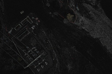 |
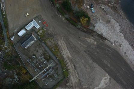
| Figure : Image and its “difference of Gaussian” at scale 10 pixels. The numerical values of the difference being small (between 0 and 40), the histogram has been modified. | |
For example, on this image of our Lac Noir site, we have applied a Gaussian filter of scale σ = 10 pixels. We have then taken the difference between the blurred image and the original. As can be seen, edges and salient points become clear.
A search for scale-space extrema is then carried out, in relation to their 26 nearest neighbours (geometrical neighbours belonging to the difference of Gaussians of the point, and also to the preceding and following differences).
A “keypoint” D (x, y, σ) is then defined by its position and also by its scale. The use of an image pyramid is recommended in order to reduce the computation time for the blurred images.
Improved coordinates of candidate points are then calculated by interpolation; points with low contrast are then eliminated, as are those on edges (which are considered to be unstable). Thus the keypoints of the image are selected .
The next stage is to calculate a descriptor for each keypoint; the matching process follows.
We begin by assigning an orientation θ to the point, starting from the direction of local gradients; this is an essential step. In effect the descriptor is calculated as a function of this orientation, which renders the method rotation-invariant. At this stage the points are defined by (x, y, σ, θ).
The descriptor as such is then calculated, taking account of a region of 16 × 16 pixels centred on the keypoint, divided into sub-regions of 4 × 4.
Different processes are carried out on the histograms of these 16 sub-regions; the final descriptor is a vector with 128 elements.
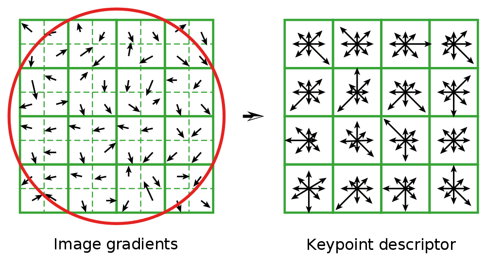 |
| Figure : SIFT descriptor(Lowe 2004) |
These detectors are used in order to place the images into correspondence. For a given point, the most probable match is that which is closest in terms of Euclidean distance. Since this operation does not take account of the geometry of objects, it obviously gives rise to numerous matching errors; moreover some points do not have matches in other images.
If at least three close points are detected as homologous, these are considered as more likely to be correct than a single point. Such clusters are used to verify the consistency of the geometrical model. In this way, the match is validated or rejected.
Once the coordinates of the camera positions in 3D space are known, we attempt to obtain a dense point cloud. Correlation techniques enable us to solve this problem. The aim is to project the pixels from multiple photos in three dimensional space. Knowing the position and calibration of the camera, it is also known that any pixel, the camera and the corresponding object point lie on a straight line. Only the distance is now required. This is found with the aid of neighbouring images.
A correlation coefficient is calculated between the numerical values of the images of a point for every position on the straight line. The position where the value of the correlation coefficient is greatest is then the most probable position of that point.
By repeating this operation for every pixel on the photos concerned, and eliminating those for which the correlation coefficient falls below a certain threshold, a dense point cloud is produced.
Note that to perform this correlation it is necessary for the photographs to overlap.
Contact
Follow us
|
|
ZA Champ du roy. 219 chem. des goules 38670 Chasse-sur-rhône |